Spatial Projections of a randomForest model

In this workshop, we will create a spatial projection of our random forest model for monthly methane exchange from natural ecosystems.

To date, we have completed model calibration, validation, and sensitivity analysis. Next, we can apply the model to a landscape to estimate natural methane emissions. For this workshop, we will calculate Connecticut’s natural emissions.

In this workshop, we will:

Make a list of the variables, their units, and the exact name and class of each variable in your model.
Determine where you can get a spatial version of each variable in your model.
Format each spatial layer to match the exact conditions of the data used to fit the model.
Make spatial predictions.
Use predictions to calculate an annual budget.

Load libraries:

library(randomForest)
library(tidyverse)
library(tidyterra)

(1) Make a list of the variables, their units, the exact name and class of each variable in your model.

Datasets: data.zip

Load the datasets and the model.

load(file="data/final_model.RDATA" )

There are four items in this.RDATA file.
(1) the randomForest model,
(2) the flux net dataset,
(3) the training data, and
(4) the testing data.

Look at the model to determine which variables are in it:

FCH4_F_gC.rf


Call:
 randomForest(formula = FCH4_F_gC ~ P_F + TA_F + Upland, data = train,      keep.forest = T, importance = TRUE, mtry = 1, ntree = 500,      keep.inbag = TRUE) 
               Type of random forest: regression
                     Number of trees: 500
No. of variables tried at each split: 1

          Mean of squared residuals: 4.40718
                    % Var explained: 32.54

The model includes precipitation in mm (P_F), mean air temperature in degrees Celsius (TA_F), and an indicator for upland ecosystems (Upland).

Check the class of each variable.

class(train$P_F)

[1] "numeric"

class(train$TA_F)

[1] "numeric"

class(train$Upland)

[1] "factor"

To project this model in space, we need the following variables:

Monthly total precipitation in mm and the name of the layer needs to be “P_F”
Monthly mean air temperature in degrees Celsius and the layer name needs to be “TA_F”
We need an indicator for upland ecosystems called Upland. All inundated ecosystems (+ snow) are given the value “0” and non-inundated ecosystems are given the value “1”. Croplands and urban areas should be filtered out of this layer.

(2) Determine where you can get a spatial version of each variable in your model.

We will spatialize the model for Connecticut in the year 2021.

Monthly total precipitation (mm): Terra climate (getTerraClim()).
Monthly mean air temperature temperature in degrees Celsius: Terra climate (getTerraClim()).
Indicator for Upland ecosystems (Upland): MODIS Land Cover Data (Majority_Land_Cover_Type_1). downloaded from: (2001 - 2022) https://lpdaac.usgs.gov/products/mcd12c1v061/ the user guide is available here: https://lpdaac.usgs.gov/documents/101/MCD12_User_Guide_V6.pdf.

To use raster layers with the predict function, they must have the same CRS, resolution, and extent!

#(3) Format each spatial layer. Download the climate layers needed for P_F and T_F using getTerraClim().

library(AOI)
library(climateR)
library(terra)
library(tidyverse)

Create an AOI for Connecticut.

ct <- AOI::aoi_get(state="CT")
plot(ct$geometry)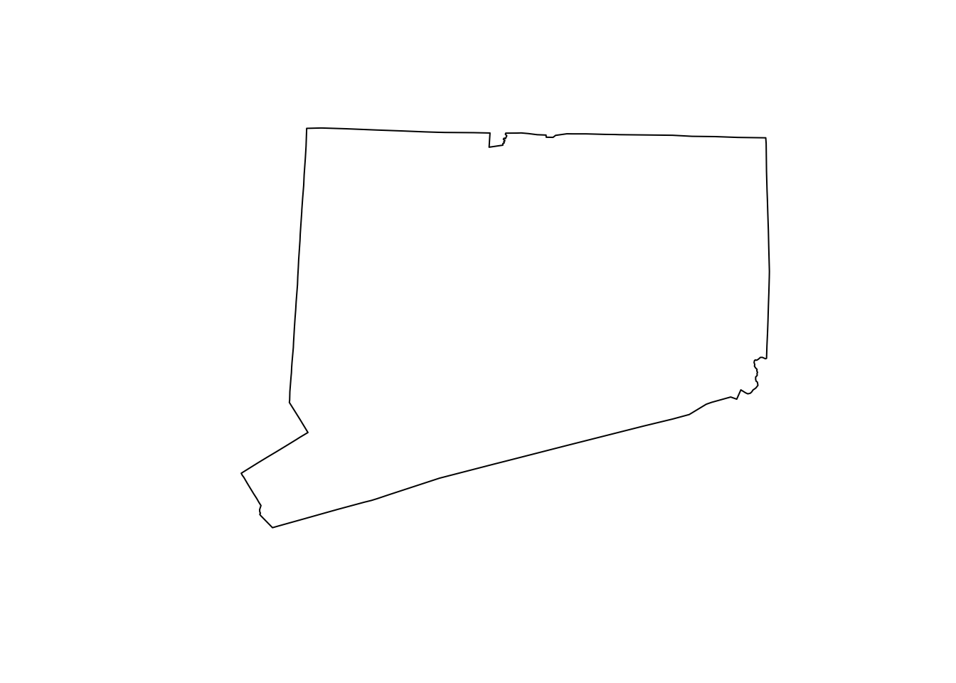

Download terra climate data (Precipitation and air temperature) for 2021.

global.clim.N <- ct %>% getTerraClim(varname = c("ppt", "tmin", "tmax"), 
                                     startDate = "2021-01-01",
                                     endDate = "2021-12-31")

Subset the data for each variable.

global.clim.ppt <- global.clim.N$ppt
global.clim.tmin <-global.clim.N$tmin
global.clim.tmax <- global.clim.N$tmax

We need mean air temperature. Calculate the mean using the maximum and minimum air temperature.

global.clim.tmean <-   mean(global.clim.tmin, global.clim.tmax)
global.clim.tmean

class       : SpatRaster 
dimensions  : 28, 48, 13  (nrow, ncol, nlyr)
resolution  : 0.04166674, 0.04166679  (x, y)
extent      : -73.75, -71.75, 40.91667, 42.08334  (xmin, xmax, ymin, ymax)
coord. ref. : +proj=longlat +ellps=WGS84 +no_defs 
source(s)   : memory
names       : tmin_~total, tmin_~total, tmin_~total, tmin_~total, tmin_~total, tmin_~total, ... 
min values  :       -5.00,        -5.9,         1.3,        7.05,       12.20,       18.65, ... 
max values  :        1.55,         1.3,         6.0,       11.15,       15.75,       22.00, ... 
time        : 2021-01-01 to 2022-01-01 UTC

Rename the layers to start with “tmean” to match the data.

names(global.clim.tmean) <- gsub(pattern = "tmin", replacement = "tmean", x = names(global.clim.tmean))
global.clim.tmean

class       : SpatRaster 
dimensions  : 28, 48, 13  (nrow, ncol, nlyr)
resolution  : 0.04166674, 0.04166679  (x, y)
extent      : -73.75, -71.75, 40.91667, 42.08334  (xmin, xmax, ymin, ymax)
coord. ref. : +proj=longlat +ellps=WGS84 +no_defs 
source(s)   : memory
names       : tmean~total, tmean~total, tmean~total, tmean~total, tmean~total, tmean~total, ... 
min values  :       -5.00,        -5.9,         1.3,        7.05,       12.20,       18.65, ... 
max values  :        1.55,         1.3,         6.0,       11.15,       15.75,       22.00, ... 
time        : 2021-01-01 to 2022-01-01 UTC

Remove the layers you no longer need.

rm(global.clim.tmin, global.clim.tmax)

Save the layers.

writeRaster(global.clim.tmean, "data/TERRA_TMEAN_2021_CT.tif", overwrite=TRUE )
writeRaster(global.clim.ppt, "data/TERRA_PPT_2021_CT.tif", overwrite=TRUE )

Now, we need to get the MODIS IGBP layers. The dataset provided was developed from MODIS Land Cover Data (Majority_Land_Cover_Type_1) downloaded from: (2001 - 2022) https://lpdaac.usgs.gov/products/mcd12c1v061/. This dataset was downloaded for the entire globe and cropped to include only Connecticut.

Load the data.

igbp.ct <- terra::rast("data/MODIS_IGBP_2001-2022_CT.tif")
igbp.ct

class       : SpatRaster 
dimensions  : 22, 39, 22  (nrow, ncol, nlyr)
resolution  : 0.05, 0.05  (x, y)
extent      : -73.75, -71.8, 40.95, 42.05  (xmin, xmax, ymin, ymax)
coord. ref. : lon/lat Unknown datum based upon the Clarke 1866 ellipsoid 
source      : MODIS_IGBP_2001-2022_CT.tif 
names       : Major~ype_1, Major~ype_1, Major~ype_1, Major~ype_1, Major~ype_1, Major~ype_1, ... 
min values  :           0,           0,           0,           0,           0,           0, ... 
max values  :          14,          13,          14,          14,          14,          13, ... 
time (raw)  : 992563200 to 1655251200

igbp.ct[[1]] %>% plot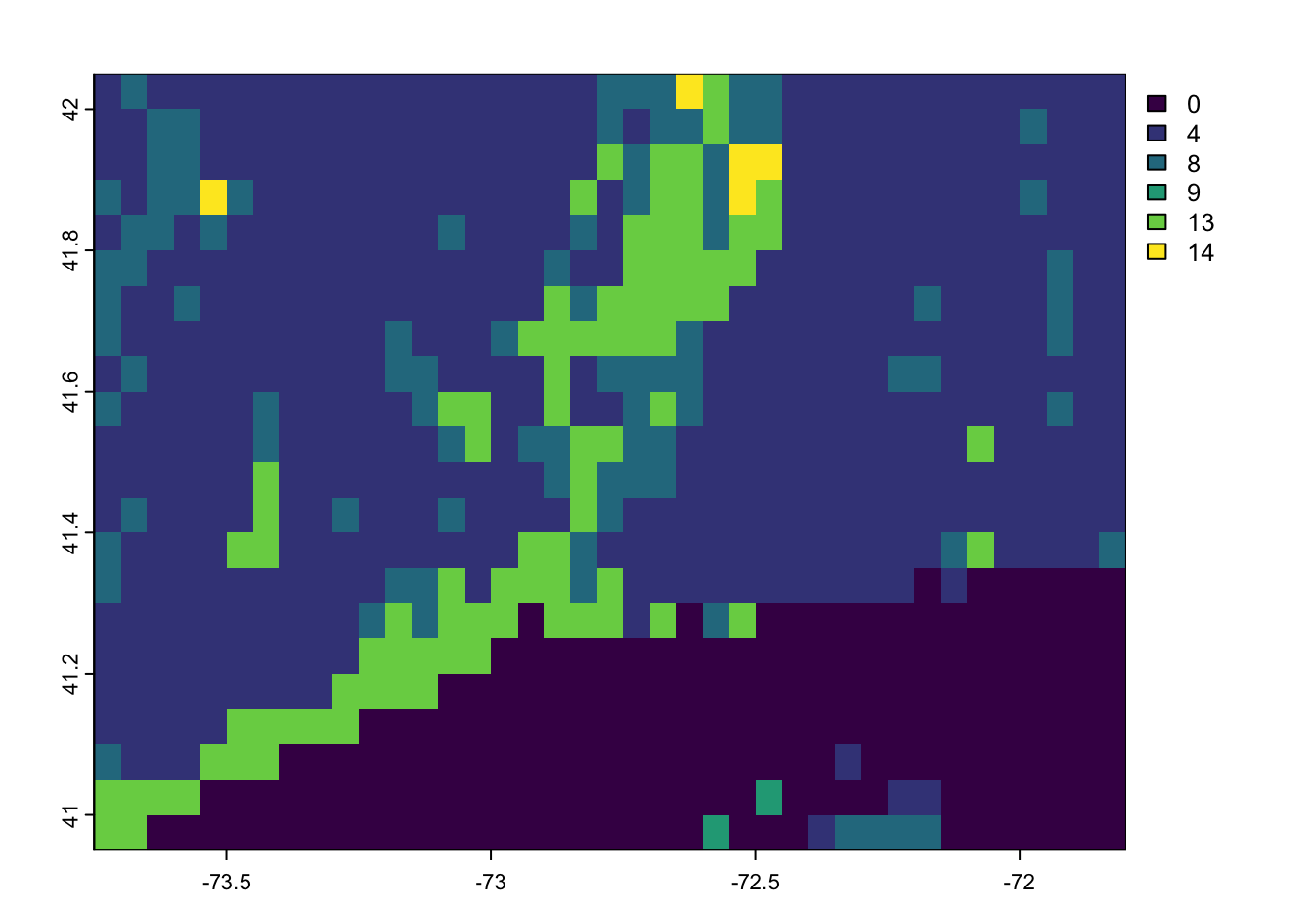

This layer needs to be reformatted. Using the User Guide we can determine what each numerical value represents: https://lpdaac.usgs.gov/documents/1409/MCD12_User_Guide_V61.pdf

1: ENF. 2: EBF. 3: DNF. 4: DBF. 5: MF. 6: CS. 7: OS. 8: WS. 9 : SAV. 10 : GRA. 11: WET. 12 : CRO. 13 : URB. 14 : CRO. 15 : SNO. 16: Barren. 17 : WAT. 0: Unclassified.

look at the layer. Here I use”[[1]]” to see only the first layer, which is for the year 2001.

terra::plot(igbp.ct[[1]])

Reclassify each value, one at a time, and think about how you should reclassify each. We want to give all uplands the value “1” and all inundated systems the value “0”.

First, make a copy of the raters (igbp.ct) and call it igbp.ct.r:

igbp.ct.r <- igbp.ct

Reclassify 0 value to NA.

igbp.ct.r[ igbp.ct.r == 0] <- NA 
terra::plot(igbp.ct.r[[1]] )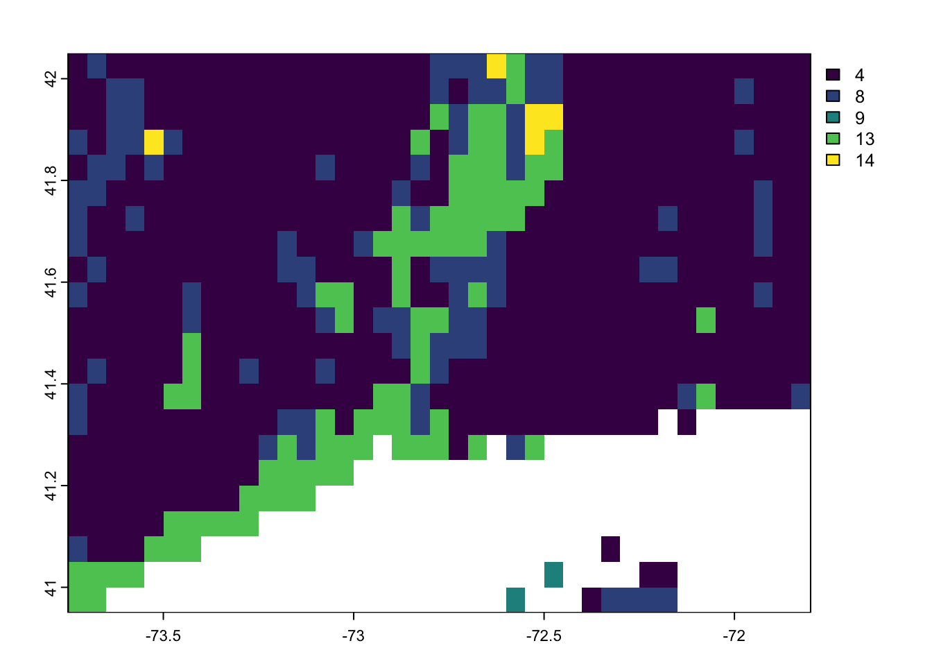

Reclassify the other values:

igbp.ct.r[ igbp.ct.r == 1] <- 1 
igbp.ct.r[ igbp.ct.r == 2] <- 1
igbp.ct.r[ igbp.ct.r == 3] <- 1
igbp.ct.r[ igbp.ct.r == 4] <- 1
igbp.ct.r[ igbp.ct.r == 5] <- 1
igbp.ct.r[ igbp.ct.r == 6] <- 1
igbp.ct.r[ igbp.ct.r == 7] <- 1
igbp.ct.r[ igbp.ct.r == 8] <- 1
igbp.ct.r[ igbp.ct.r == 9] <- 1
igbp.ct.r[ igbp.ct.r == 10] <- 1
igbp.ct.r[ igbp.ct.r == 11] <- 0
igbp.ct.r[ igbp.ct.r == 12] <- NA
igbp.ct.r[ igbp.ct.r == 13] <- NA
igbp.ct.r[ igbp.ct.r == 14] <- NA
igbp.ct.r[ igbp.ct.r == 15] <- 0
igbp.ct.r[ igbp.ct.r == 16] <- 1
igbp.ct.r[ igbp.ct.r == 17] <- 0

Look at the final raster to ensure everything is reclassified to upland since Connecticut doesn’t have anything else at the resolution of MODIS.

terra::plot(igbp.ct.r[[1]], col='red' )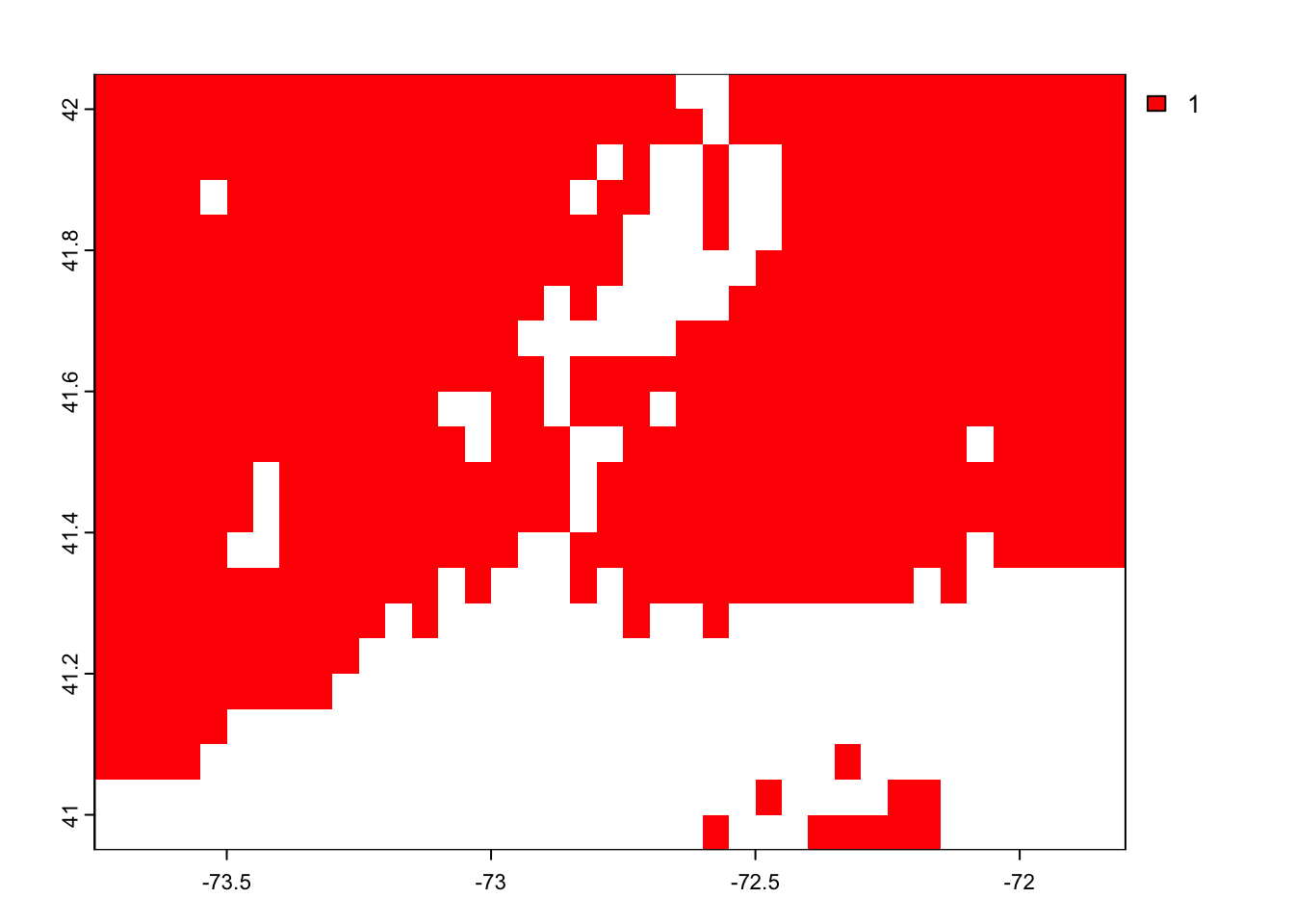

Format the upland layer as a factor by first making a data frame that has the raster values 0 and 1 and the corresponding factor level.

factors.df <- data.frame(id=c(1, 0), cover=c("upland", "inundated"))

Create a for loop to assign the factor levels to each raster layer one at a time:

for ( i in 1:22){
  print(i)
  levels(igbp.ct.r[[i]]) <- factors.df
  is.factor(igbp.ct.r)
}

[1] 1
[1] 2
[1] 3
[1] 4
[1] 5
[1] 6
[1] 7
[1] 8
[1] 9
[1] 10
[1] 11
[1] 12
[1] 13
[1] 14
[1] 15
[1] 16
[1] 17
[1] 18
[1] 19
[1] 20
[1] 21
[1] 22

terra::plot(igbp.ct.r[[1]], col="red" )

We only need the layer for 2021. Subset the 2021 layer.

igbp.ct.r.2021 <- igbp.ct.r[[21]]

We will use the CRS of the terra climate layers and make everything match this.

igbp.ct.r.2021 <- terra::project( igbp.ct.r.2021, global.clim.ppt)

All the resolutions must be the same to combine the rasters into one item. We will set the terra climate layers to match the igbp.ct.r layer:

global.clim.tmean.resample <- resample( global.clim.tmean, igbp.ct.r.2021)
global.clim.ppt.resample <- resample( global.clim.ppt, igbp.ct.r.2021)

Now, export the files to save a version processed as needed.

writeRaster(global.clim.tmean.resample, "data/products/TERRA_TMEAN_2021_CT_rs.tif", overwrite=TRUE )
writeRaster(global.clim.ppt.resample, "data/products/TERRA_PPT_2021_CT_rs.tif", overwrite=TRUE )
writeRaster(igbp.ct.r.2021, "data/products/MODIS_Upland_2021_CT.tif", overwrite=TRUE )

(4) Make predictions

Combine all the variables into a raster stack, only including one month since igbp.ct.r.2021 has one layer and the climate has 12, one for each month.

model.rasters.m1 <- c(igbp.ct.r.2021, global.clim.tmean.resample[[1]], global.clim.ppt.resample[[1]] )

If you have any issues combining the raster layers into one object, you may not have made everything the same resolution or extent.

Make the names of the raster layers match the dataframe.

names(model.rasters.m1 ) <- c("Upland", "TA_F", "P_F" )
model.rasters.m1

class       : SpatRaster 
dimensions  : 28, 48, 3  (nrow, ncol, nlyr)
resolution  : 0.04166674, 0.04166679  (x, y)
extent      : -73.75, -71.75, 40.91667, 42.08334  (xmin, xmax, ymin, ymax)
coord. ref. : +proj=longlat +ellps=WGS84 +no_defs 
source(s)   : memory
names       : Upland,  TA_F,  P_F 
min values  : upland, -5.00, 41.2 
max values  : upland,  1.55, 65.6 
unit        :       ,      ,   mm

Check the dataframe again to ensure you don’t need to make additional changes to the raster.

class(train$Upland )

[1] "factor"

summary(train$Upland )

inundated    upland 
      974       697

levels(train$Upland )

[1] "inundated" "upland"

model.rasters.m1$Upland

class       : SpatRaster 
dimensions  : 28, 48, 1  (nrow, ncol, nlyr)
resolution  : 0.04166674, 0.04166679  (x, y)
extent      : -73.75, -71.75, 40.91667, 42.08334  (xmin, xmax, ymin, ymax)
coord. ref. : +proj=longlat +ellps=WGS84 +no_defs 
source(s)   : memory
categories  : cover 
name        : Upland 
min value   : upland 
max value   : upland

You are ready to use the predict function to predict you model in space.

model.rasters.m1.pred <- terra::predict(  object= model.rasters.m1, model=FCH4_F_gC.rf)

plot(model.rasters.m1.pred)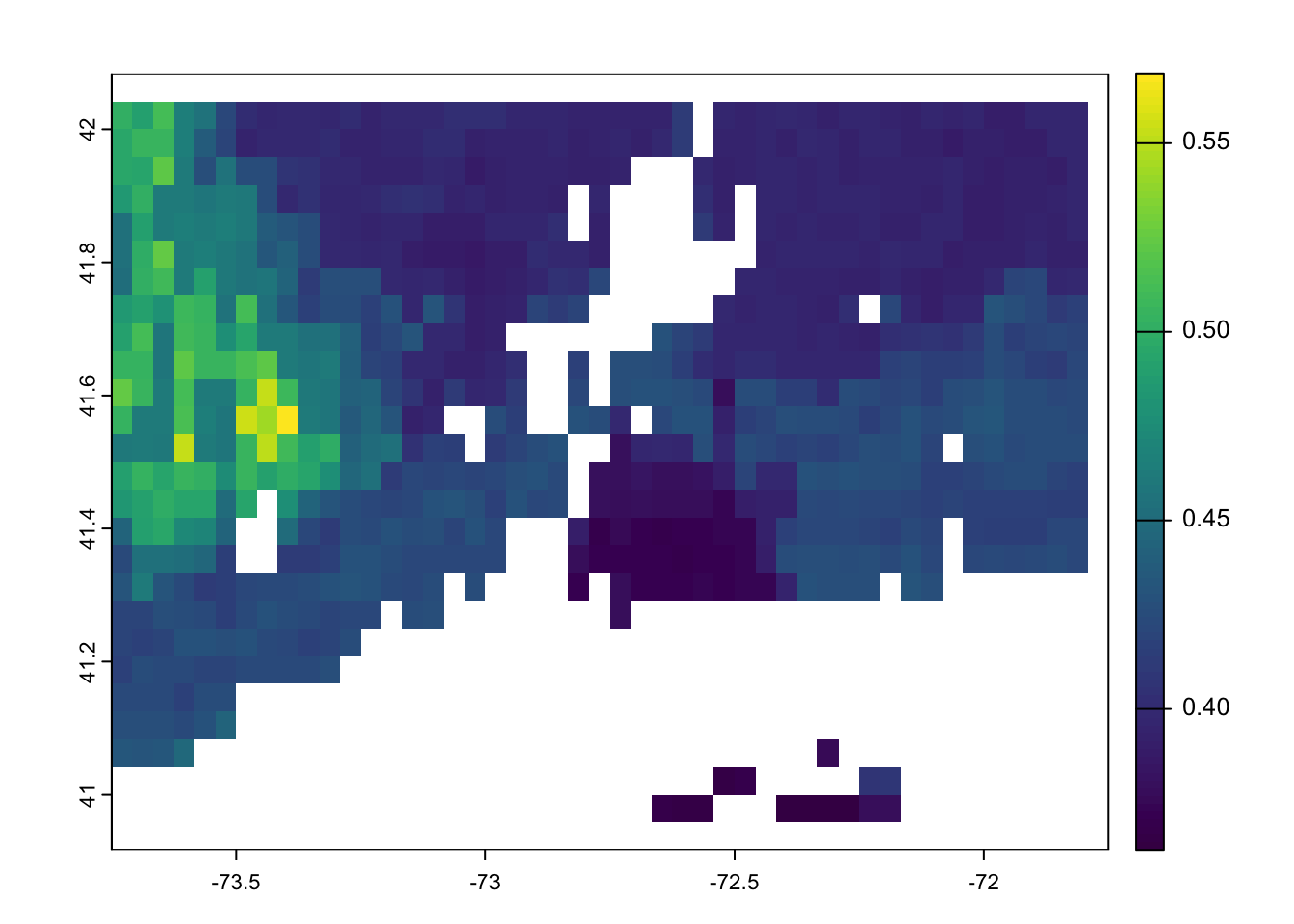

We can do this in a for loop to get all 12 months.

First, determine where you want to export the files to, and make a new folder there called predictions.

setwd('data/products/') # sets the working directory to your products folder
directory <- getwd() # saves the path to directory
subDir <- 'predictions' # You will use this to make the folder called predictions

dir.create(file.path(directory , subDir)) # this makes the new folder in data called predictions

Warning in dir.create(file.path(directory, subDir)):
'/Users/ac3656/GitHub/EDS_course/data/products/predictions' already exists

predictions.dir <- paste(directory,"/",subDir, sep="")

Make the forloop to make predictions for all 12 months.

for ( i in 1:12){
 
  print(i)
  
  model.rasters <- c(igbp.ct.r.2021, global.clim.tmean.resample[[i]], global.clim.ppt.resample[[i]] )
  names(model.rasters) <- c("Upland", "TA_F", "P_F" )
  pred <- terra::predict(  object= model.rasters, model=FCH4_F_gC.rf)
  
  units(pred) <- 'g C m-2 month-1' # Add the units
  names(pred ) <- "F_CH4" # Name the layer
  
  writeRaster(pred ,paste(predictions.dir,"/","MODEL_PRED_m",i,".tif", sep =""), overwrite=TRUE )
}

Delete the json files created:

setwd(predictions.dir)
delete <- list.files( path = predictions.dir, pattern=".json")
file.remove(delete)

logical(0)

Make of list of all the files in a directory that you want to import, and import all the files in the list with rast().

setwd(predictions.dir)
pred <- list.files( path = predictions.dir, pattern="MODEL_PRED_m")
predictions <- rast(pred)

(5) Use predictions

Create the 2021 methane budget. To get an annual budget, sum the total monthly fluxes.

predictions.2021.total <- sum(predictions )
units(predictions.2021.total ) <- 'g C m-2 year-1' # add the units
names(predictions.2021.total ) <- "F_CH4"

To determine the total amount of methane in 2021 for natural areas we need to consider the area:

ct.area = cellSize(predictions.2021.total, unit="m")
predictions.2021.total$F_CH4_total <- (predictions.2021.total$F_CH4 * ct.area)/1000000000000 
units(predictions.2021.total$F_CH4_total) <- "Gigatons of carbon per year"

# Total emissions in 2021:
global( predictions.2021.total$F_CH4_total, "sum", na.rm=T)

                  sum
F_CH4_total 0.1154527

Now you are ready to follow the same workflow for your model. (1) For your final project, determine where you will project your model.
(2) Make a list of the variables, their units, the exact name and class of each variable in your model.
(3) Determine where you can get a spatial version of each variable in your model.
(4) Format each spatial layer. (5) Make predictions. (6) Use predictions.

Ensure your raster layers all have the same CRS and resolution!